Laying of linear infrastructure in TeleCAD-GIS
There are two (slightly different) approaches to laying linear infrastructure
in TeleCAD-GIS.
- Laying from object to object (with the possibility to select the via-points).
- Laying from route-point to route-point.
1. Laying from object to object refers to:
- Duct bank
- Copper cables
- Fiber optic cables
- Coaxial cables
2. Laying from route-point to route-point refers to:
- Innerducts
- Crossing ducts
- Abandoned cables (copper, fiber optic...)
All infrastructure in TeleCAD-GIS is laid along the routes (TCG object
- route).
The user selects route-points or nodal elements to connect with the infrastructure,
and the program automatically connects them using the shortest possible
path along the predefined routes.
The drawing prepared for laying of linear infrastructure (Figure 1) contains the routes and nodal elements of infrastructure (only routes for the second case).
| Note: |
Nodal element symbol is arbitrarily shown as a pentagon and replaces the display of elements such as distribution terminal, manhole, splice point, telephone exchange etc. |
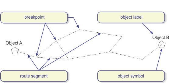
Figure 1
1. Laying from an object to an object
Laying from an object to an object refers to:
- Duct bank
- Copper cables
- Fiber optic cables
Laying along the shortest path
If you want to lay the linear infrastructure, so that its position is as in Figure 2 (green line),

Figure 2
then the procedure is as follows.
From the main menu run one of the commands for laying the linear infrastructure.
The cursor is in the form of a small rectangle, and the program expects
you to select the nodal element of the network.
Select Object A by clicking on its symbol or on its label. Then, select
Object B.
Objects are connected along the route using the shortest
possible path.
Temporary red line is displayed, showing where the future duct bank will
be.
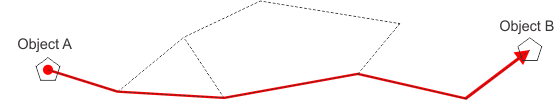
Figure 3
Complete the command by right-clicking or pressing the ENTER key.
Linear infrastructure is generated (blue line - Fig. 4).

Figure 4
Laying along the arbitrary path ("via" points)
If you want to lay the linear infrastructure, so that its position is as in Figure 5 (green line),
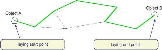
Figure 5
then the procedure is as follows.
From the main menu run one of the commands for laying the linear infrastructure.
The cursor is in the form of a small rectangle, and the program expects
you to select the nodal element of the network.
Select Object A by clicking on its symbol or on its label.
At this point, while the command is active, you can see an additional
command option [t] in the command line.
This option offers you the possibility to select via-points. The option
is triggered by typing the letter "t" on your keyboard.
The cursor changes shape to a "+" sign and you can now select
the route-point.
After selecting the via-point, Object A and via-point are connected by
the shortest path
(the program displays a temporary red line between Object A and via-point
T).
The cursor is again in the form of a small rectangle, and the program expects
you to select the nodal element of the network.
(Note: If you want to select another via-point, type "t" once
again on your keyboard)
At the end, select Object B.
Via-point T and Object B are connected by the shortest possible path.
Temporary red line is drawn, showing where the future linear infrastructure
will pass.

Figure 6
End the command by right-clicking or pressing the ENTER key.
Linear infrastructure is generated (blue line - Fig. 7).

Figure 7
When laying the infrastructure along an arbitrary path, it is possible
to assign more via-points that determine the path.
The following example illustrates importance of the order when selecting
via-points.
If you want to lay the linear infrastructure, so that its position is as in Figure 2 (green line),

Figure 8
then the procedure is as follows.
From the main menu run one of the commands for laying the linear infrastructure.
Select Object A, then via-point T1, via-point T2 and finally Object B.

Figure 9
End the command by right-clicking or pressing the ENTER key.
Linear infrastructure is generated (blue line - Fig. 4).
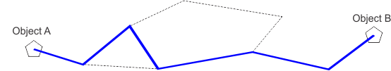
Figure 10
It is incorrect to select the first via-point T1 at the position as
shown in Figure 8,
and then select the second via-point T2 and lastly Object B.

Figure 11
In that case, the infrastructure overlaps at the route segment between points T1 and T2 (Fig. 9).

Figure 12
When checking the topology (Automatic route correction command or when sending to database), the program reports the infrastructure laid in this way as an error.
2. Laying from route point to route point
Laying from route point to route point refers to:
- Innerducts
- Crossing ducts
Procedure
From the main menu run one of the commands for laying the linear infrastructure.
The cursor is in the form of a "+" sign, and the program expects
you to select the route-point.
By clicking on the route-point, select the first point (from which you
want the infrastructure to start),
then select via-points (through which the linear infrastructure will pass)
and in the end select the point at which you want the infrastructure to
end (Figure 13).

Figure 13
| Note: |
1. It is enough just to select the start and the end point.
In that case, they will be connected along the shortest possible
path. |
Selected points are connected along the shortest possible path and in the
order they were selected.
Temporary red line is drawn, showing where the future linear infrastructure
will pass.
Complete the command by right-clicking or pressing the ENTER key.
Linear infrastructure is generated (blue line - Fig. 14).
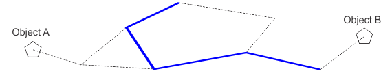
Figure 14
If you want to lay such linear infrastructure from the nodal element
of the infrastructure (manhole, distribution terminal, OTB and similar),
just select the route-point at which the nodal element is set (e.g. route
point at which Object A is set - Fig. 15).
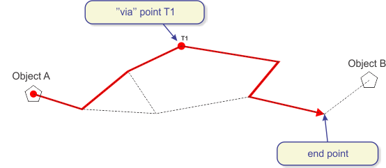
Figure 15
Linear infrastructure is generated (blue line - Fig. 16).

Figure 16