Window: DB Optic View

DB Optic View window is opened by running TCG Map - Optics
command. It enables an overview of all fiber optics elements entered into GIS database, creating a schematic display of all the selected elements and loading of elements displayed on the scheme into the site plan.

DB Optic View window provides a view into the current status of GIS database.

The view is enabled in two ways:

• View in the form of infrastructure shown on the geographical map.
  It shows a complete optics infrastructure in GIS database.
• View in the form of the schematic display of the selected part of infrastructure.
  It shows a part of fiber optics infrastructure selected by the user and loaded into the schematic display.

Window: DB Optic View

DB Optic View  window is opened by running TCG Map - Optics command (Figure 1).

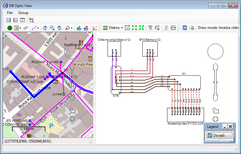
Figure 1

DB Optic View window contains the following items:

• Main menu
• Toolbar
• Map (with its own toolbar)
• Schematic display (with its own toolbar)

Main menu

The main menu contains the following commands:

• File
  • View
    • - Save View
      By running this command, the current position on the map will become the default one.
      This means that each time DB Optic View window is opened again we will be in the area.
    • - Drawing -> Map
      Let us assume that we are in a dwg drawing with a loaded infrastructure from the database.
      One of the infrastructure elements is the ODF. The easiest way to find the ODF in DB Optic View is to position the ODF in the drawing and click  Drawing -> Map after opening DB Optic View.
    • - Map -> Drawing
      Let us assume that we are in DB Optic View window.
      By using  Pan (pressing the mouse wheel) and Zoom (rolling the mouse wheel) tools we have moved around the map and now we are at the main Post Office at Takovska Street (Belgrade).
      If we also want to be in the same location in the drawing, we should click  Map -> Drawing
      . After this the working space of the drawing shall also be placed in the coordinates of the main Post Office.
  • - Db Info
    Opens the window with basic information on GIS database we are currently connected to (primarily intended for administrators).
  • - Export to Drawing
    Loads all the elements in the site plan which are loaded in the schematic display (see  Load Optics from GIS Database).
  • - Export Selected to Drawing
    Loads all the elements in the site plan which are loaded in the schematic display, but only those selected by the user in the schematic display (see  Load Optics from GIS Database).
• Group
  • - Open - Opens the scheme saved as *.ischX file
  • - Save - Saves the scheme saved as *.ischX file
  • - Delete - Removes all the elements from the schematic display (deletes the scheme)

Toolbar

The toolbar contains the following tools:

• - Map
  Shows the map only (during the opening of DB Optic View window, the default status implies only the opened map).
• - Scheme
  Shows the schematic display only.
• - Map|Scheme
  Shows both the map and schematic display comparatively.
• - Create Scheme from Marked Objects
  Loads elements from the basket. The basket should previously be filled with network elements from GIS database.
  The procedure is described in detail on Load Optics from GIS Database page.

Map

The map shows all the fiber optics infrastructure entered into GIS database (Figure 2).

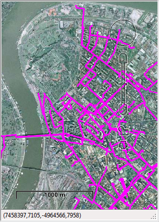
It is used to overview and load infrastructure (loading is described in detail on Load Optics from GIS Database page).

Map context menu commands

The context menu is opened by right-clicking on one of the elements shown on the map (cable, splice point, distribution frame, manhole).

Right-clicking on any of the cables can run the following command:

• Show on Scheme - The selected cable gets selected on the scheme
• Cable Fibers - Opens Fiber Info window which shows detailed information on all the fibers of the observed cable
• Route Trace - Additional commands related to Fiber Trace tool
  • Avoid Node - Adds the cable to the “Avoid” list
  • Remove Node - Removes the cable from the list, whether it is “Route” or “Avoid” list

Right-clicking on any of fiber optics nodal elements can run the following command:

• Show on Scheme - The selected nodal element gets selected on the scheme
• Node Fibers - Opens Fiber Info window which shows detailed information on all the fibers of the observed nodal element
• Route Trace - Additional commands related to Fiber Trace tool
  • Add to Route - Add the nodal element to the list of points between which the route is sought (“Route” list)
  • Avoid Node - Adds the nodal element to the avoid list
  • Remove Node - Removes the cable from the list, whether it is “Route” or “Avoid” list

Right-clicking on any manhole can run the following commands:

• Open Manhole Opens the manhole butterfly diagram
• Show on Scheme - The selected manhole gets selected on the scheme

Toolbar (map)

The map has its own toolbar with the following tools:

• - Indicator - Map loading progress indicator (=loaded; =loading in progress)
• - Map - Enables the selection of cartographic material sources  (basemaps) from the drop-down menu.
• - Display Mode - When this icon is open, all the elements are shown on the map
• - Display Mode - When this icon is open, only those elements on the scheme are shown on the map
• - Display Method - Enables the selection of one of the possible methods of infrastructure display (see more detailed)
• - Site Plan View
• - GIS View
• - Resolve Overlaps
• - Previous Zoom - Returns to the previous zoom
• - Zoom to Area - Enables zooming to the  mouse-encompassed area (zoom window)
• - Next Zoom - Next zoom
• - Select/Move Control
  Set of commands controlling the way the map/scheme working space behaves when using the following commands: Show on Scheme, Show Cable on Site Plan or Show Nodal Element on Site Plan
• - Select - (the element will be selected, no working space zooming or moving)
• - Select+Zoom  - (the element will be selected and the zoom such that the whole element is visible) (default status)
• - Select+Move  - (the element will be selected, the zoom does not change, and the working space moves so that the selected element comes into the center of the display)
  (the last comes in handy when a nodal element should be displayed; when the cable is displayed, it does not make much sense, for it be positioned in the cable center)
• - Add to Basket - Adds network elements selected on the map to the basket.
  The elements in the basket are loaded into the scheme by means of Create Scheme from Marked Objects () command.
  (See procedure on Load Optics from GIS Database page.)
• - Remove from Basket - Removes network elements selected on the map from the basket.
• - Additional Tools - Opens the window which shows the following tools:
• Fiber Trace (see more detailed)
• FO Paths (see more detailed)

Shematic Display

The schematic display shows network elements selected by the user on the map and loaded into the scheme (Figure 3).
The elements (cables, nodal elements...) are shown schematically.

Since it is almost the same as the schematic display of TCG Optic View (DWG) window, it is described along with it on Window:TCG Optic View (DWG) page (the differences are particularly emphasized).

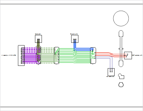
Figure 3

Toolbar (schematic display)

The schematic display has its own toolbar.
The schematic display toolbar is also quite similar to the one in TCG Optic View (DWG) window.
It is described in detail on Window: TCG Optic View (DWG) page (the differences are particularly emphasized).