Window: TCG Optic View (DWG)
- Display modes of schematic diagram
- Splicing
- Differences between windows:
"TCG Optic View (DWG)" and schematic
display in "DB Optic View" window
- The main difference:
- The difference in toolbar commands
- The difference in the commands that are opened by right-clicking on a linear infrastructure element (cable or fiber) in the schematic display
- The difference in the commands that are opened by right-clicking on the nodal element (splice point or distribution frame) in the schematic display
- Difference: Splicing
- The difference in "incomplete fibers" display
| Introduction note: |
| On this page we’ve primarily described TCG
Optic View (DWG) window. However, as the schematic diagram on the window DB Optic View is almost exactly the same, all that is said here applies to it as well. Some commands are different, or are in one case active and in the other not. The differences are listed below (in the notes) and additionally listed at the end of the page. The main difference is that the window TCG Optic View (DWG) is a schematic diagram of the optical network infrastructure that is located in the site plan drawing, and the schematic diagram on the window DB Optic View refers to the infrastructure that is in the GIS Database (a direct view into the GIS Database). |
Window TCG Optic View (DWG) shows
all the elements of the optical network that are in the site plan drawing.
The elements (cables, ODF, OTB, Patch Panel ...) are shown schematically.
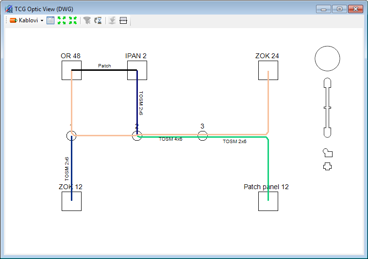
Figure 1
We use this window to overview the infrastructure, analyze, detect errors,
and to start the process of fiber splicing.
If we set all the elements of the network (with no splicing) in the site
plan drawing, then almost all the work related to the FO network can be
done in the schematic diagram.
Navigating through the schema
Navigating the schema is done using the mouse or the navigation tools
in upper right corner of the schema workspace.
Mouse is used in a standard way:
- By scrolling the mouse wheel we can zoom in and zoom out
- By pressing the mouse wheel we can move the workspace (Pan)
- Double-clicking on the mouse wheel displays the entire schema (zoom extents)
- If schema elements are selected using rectangular selection area
(pressed left mouse button while defining the area),
then all the elements touched by the selection rectangle will be selected when dragging the cursor to the left.
If the cursor is dragged to the right, only those elements completely encircled by the selection rectangle will be selected. - Several elements can be selected at once using the left-click while the SHIFT key is pressed.
Toolbar
Schematic display has its own toolbar with the following tools:
- Drop-down list
from which we select the schema display mode (explained in more detail
below on this page):
 - Show Docker
Displays the legend and additional tools if you are in the fiber display mode (more on the Docker page)
 - Increase space between
elements
- Increase space between
elements
Moves apart elements of the schema to improve the clarity, we use it if there are a lot of elements displayed
 - Reduce distance between
elements
- Reduce distance between
elements
Brings elements of the schema closer together.
 - Turn off filter
Removes any applied filters, i.e. shows the full schema (with all elements)
(Filtering is done using commands such as Show fibers of this cable and the like.)
 - Last loaded element
Marks the element that was last loaded from the GIS database.
(The command is only active in the DB Optic View window.)
 -
Export to block
-
Export to block
This command is described on the page Command: Export to block
(Command is active only in the TCG Optic View (DWG) window.)
 - Manholes (display manholes mode)
This command allows you to add manholes to the schematic diagram:- Remove manholes
Removes all manholes from the schematic diagram. - Add only
manholes with FO elements
Only manholes containing some nodal element of the FO network are added to the existing schema. - Add all manholes
through which the FO cable is passing
All manholes through which FO cables displayed in the scheme are passing are added to the existing schema.  - Select the element you
want to locate in the scheme:
- Select the element you
want to locate in the scheme:
Allows you to locate the object in the schema by selecting that same object in the site plan drawing, i.e. navigating the schema using the site plan drawing.
By clicking on an element in the site plan drawing, that same element is selected in the schema. This tool is fully operational in "Cables" and “FO Paths" modes (you can locate both cables and nodal elements), while in the "Edit schema display" mode you can locate only nodal elements. You cannot use this tool in “Fibers" mode .
 - Refresh
Refreshes the schema according to the settings in the Docker (see details).
 - Refresh
fiber connectiviry
- Refresh
fiber connectiviry
Refreshes information about the fiber splicing (see details).
- Draw mode: Analyze
fibers by: [applied analysis]
Indicator of applied analysis.
 - Check errors
Checks fibers and displays only those with errors (if any) (more details on Errors page).
Display modes of schematic diagram
There are 4 display modes of schematic diagram.
In one of them, and that is:
 - Edit Schema Display.
we adjust (edit) the geometry of the schema,
and the other three:
 - Cables
  - FO Paths
 - Fibers
we use to navigate the scheme, for splicing, correcting errors, analysis, overview of infrastructure etc.
Mode: Edit Schematic Display
By selecting Edit Schematic Display from
the drop-down list, enter the mode in which you can adjust the appearance
of the schema according to your own needs.
Changes made in this mode will be reflected in other three modes (Cables,
FO Paths and Fibers). In this mode, we change the geometry
of the schematic diagram elements.
The procedure is described in detail on Edit
Schematic Display page.
Mode: Cables
By selecting Cables from the drop-down list, enter the mode in which the schema displays the cables (Figure 2).
Figure 2
Each cable is displayed in a different color, and the legend window
is initially displayed in the lower right corner (Figure 3)
(if we shut down the legend (Docker), we can re-open it by clicking on
- Display Docker).
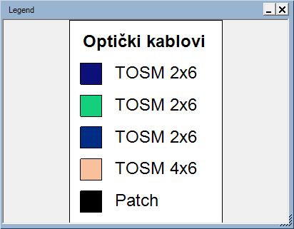
Figure 3
Commands of the context menu
By right-clicking on the cable item, you can run the following commands:
- Cable info
Opens the Cable info window (see Mode: FO Paths in the text below) - Load nodal elements
of the cable
This command loads nodal elements connected to the cable (splice points, ODFs, OTBs...).
(The command is only active in the DB Optic View window.) - Load all fibers
of this cable
This command loads all the fiber circuits passing through the cable. All elements through which the fiber circuits pass are loaded.
(The command is only active in the DB Optic View window.) - Select the cable
in site plan drawing
Selects and displays the cable in the site plan drawing. Use this command to easily locate the cable. - Show fibers of
the cable
Displays only fiber circuits passing through the selected cable together with all nodal elements through which these fibers pass/terminate (thus entering the "Fiber” mode).
Everything else gets hidden. (Return to the whole schema display by clicking on - Turn off
the filter icon.) - Show all fibers
of the FO Path
Displays all fibers of the selected cable’s FO path together with all nodal elements through which these fibers pass/terminate (thus entering the "Fiber” mode).
Everything else gets hidden. (Return to the whole schema display by clicking on- Turn off
the filter.) - Remove selected
cables from schematic diagram
Removes selected cables from the schema (only cables, if other elements are selected too). - Remove all selected
objects from schematic diagram
Removes all selected objects from the block scheme (cables, splice points, distribution frames etc.).
By right-clicking on any of the nodal
elements, you can run the following commands:
- Load all passing-through
cables
Loads all (direct) cables that pass through or terminate in the observed element.
(The command is only active in the DB Optic View window.) - Load fibers of
this nodal element
Loads all the fibers which pass through or terminate in the selected element.
By loading the fibers, all cables and all nodal elements through which these fibers pass/terminate are loaded too.
(The command is only active in the DB Optic View window.) - Select nodal
element in site plan drawing
Selects and displays the nodal elements (ODF, OTB etc.) in the site plan drawing. Use this command to easily locate the nodal element. - Display fibers
passing through this nodal element
Displays all fibers that pass through the selected nodal element together with all other nodal elements through which these fibers pass/terminate (thus entering the "Fiber” mode).
Everything else gets hidden. (Return to the whole scheme display by clicking on - Turn off
the filter.) - Remove element
from the schema
Removes selected nodal elements from the block schema.
Mode: FO Paths
By selecting FO Paths from the drop-down list, we enter the mode in which the schema displays the FO Paths (Figure 4).
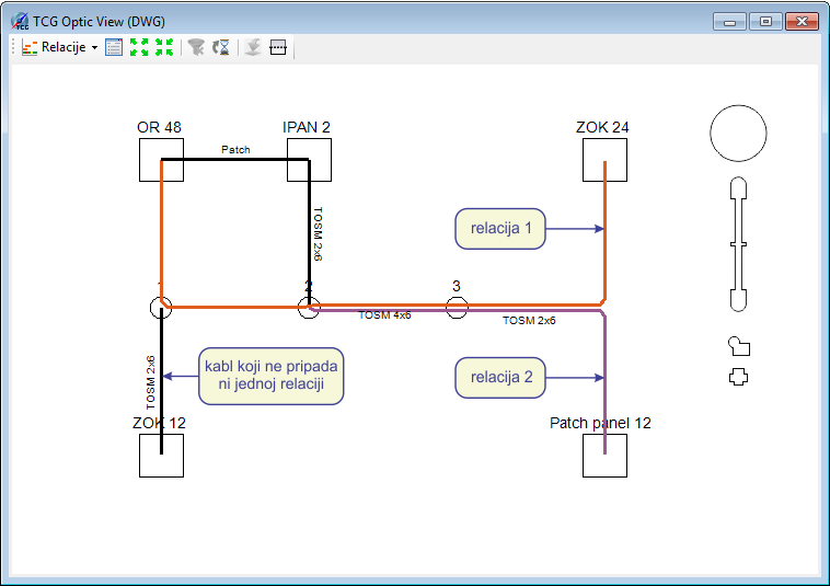
Figure 4
Cables belonging to the same FO path are displayed in the same color.
Cables that do not belong to any FO path are initially shown in black (the
user can change the colors using the legend (docker)).
The legend window (docker) is initially displayed in the right corner (Figure
5).
If we shut down the legend, we can re-open it by clicking on - Display
Docker).
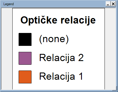
Figure 5
Commands of the context menu
By right-clicking on any of the cables, you can run one of the following commands:
- Cable
info
It opens Cable info window that we use to assign a cable to the FO path (see Assign cables to FO path). - Load all nodal
elements of the cable
This command loads nodal elements of the selected cable (splice points, ODFs, OTBs...).
(The command is only active in the DB Optic View window.) - Load fibers of
this cable
This command loads all the fiber circuits passing through the cable. All elements through which the fibers pass are loaded together with the fibers.
(The command is only active in the DB Optic View window.) - Display cable
in site plan drawing
Selects and displays the cable in the site plan drawing. Use this command to easily locate the nodal element. - Show fibers of
the cable
Displays all fiber circuits passing through the selected cable together with all nodal elements through which these fibers pass/terminate (thus entering the "Fiber” mode).
Everything else gets hidden. (Return to the whole schema display by clicking on - Turn off
the filter.) - Show all fibers
of the FO Path
Displays all fiber circuits of the selected FO path together with all nodal elements through which these fibers pass/terminate (thus entering the "Fiber” mode).
Everything else gets hidden. (Return to the whole schema display by clicking on - Turn off
the filter.) - Remove selected
cables from schema
Removes selected cables from the block schema (only cables, even if other elements are selected too). - Remove all selected
objects from schema
Removes all selected objects from the schema (cables, splice points, distribution frames etc.).
By right-clicking on any of the nodal
elements, you can run the following commands:
- Load all passing-through
cables
Loads all (direct) cables that pass through or terminate on the selected element.
(The command is only active in the DB Optic View window.) - Load all fibers
of this nodal element
Loads all the fiber circuits which pass through or terminate on the selected element.
By loading the fiber circuits, all cables and all nodal elements through which these fibers pass/terminate are loaded too.
(The command is only active in the DB Optic View window.) - Display nodal
element in site plan drawing
Selects and displays the nodal elements in the site plan drawing. - Display all fibers
passing through this nodal element
Displays all fiber circuits that pass through the selected nodal element together with all other nodal elements through which these fibers pass/terminate (thus entering the "Fiber” mode).
Everything else gets hidden. (Return to the whole schema display by clicking on - Turn off
the filter.) - Remove element
from the block schema
Removes selected nodal elements from the schematic diagram.
Mode: Fibers
By selecting the Fibers item from the drop-down list, we enter the mode in which the scheme displays fiber circuits (Figure 6).
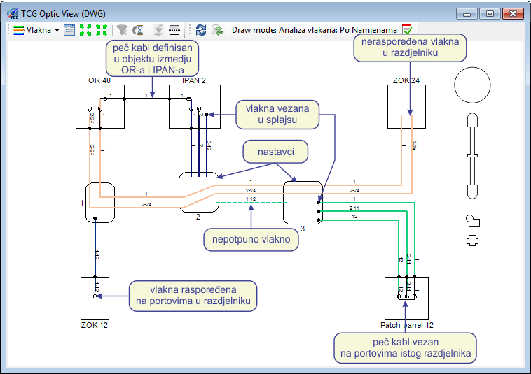
Figure 6
When we are in the Fibers
mode, in the schematic diagram we see fibers of cables that are in the
site plan drawing
(or fibers of cables loaded into the schema if we work with the DB
Optic View window).
Ways in which the fibers are displayed are defined on Docker
("Settings” tab).
At the same time, the docker is a powerful tool for analyzing the FO network
(make sure you study it).
| Tip: |
Combinations that may arise from the use of filters and analysis contained in the Docker are numerous. To take full advantage of this tool, refer to the options offered, play and experiment. First, see their description on Docker page. |
Commands of the context menu
By right-clicking on the line representing the fiber circuit or fiber circuit group, you can run the following commands:
- Fiber Info
Opens the Fiber Info window which contains two tabs: "General" and "Fiber Details".
"General" tab displays the circuit name and allows the assignment of new or change of existing circuit names.
There’s also is a list of errors on this tab, if there are any (detailed on pages Errors and Circuit Name).
„Fiber Details" tag displays various data asociated with the fiber circuit (detailed on page describing the “Fiber Details” tab).
(You can run this command by double-clicking on the line representing the fiber circuit or fiber circuit group) - Load complete
fiber circuit(s)
Command loads the selected fiber circuit (or group of fiber circuits). All elements through which the fiber circuits pass are loaded together with the fibers.
(The command is only active in the TCG Optic View window.) - Display only
selected fibers
Displays only selected fiber circuits and all nodal elements through which the fibers pass/terminate.
Everything else gets hidden. (Return to the whole schema display by clicking on the icon- Turn
off the filter.)
Multiple fiber circuits can be selected at once using the SHIFT key or by dragging the cursor to the left (you only need to touch the fiber to select it). - OTDR Trace
Opens OTDR Trace tool for working with the selected fiber circuit (described in detail on the OTDR Trace page).
By right-clicking on the nodal elements, you can run the following commands:
- Display nodal
element in site plan drawing
Selects and displays the nodal elements in the site plan drawing. Use this command to easily locate the nodal element. - Display all fibers
passing through this nodal element
Displays all fiber circuits that pass through the selected nodal element together with all other nodal elements through which these fibers pass/terminate.
Everything else gets hidden. (Return to the whole schema display by clicking on the icon - Turn
off the filter.) - Edit Element
Opens a detailed view of the selected nodal element (splice point, distribution frame etc.) and allows additional actions (primarily the splicing). - Route Trace
- Additional commands related to Fiber
Trace tool
- Add to Route - Adds a nodal element on the list of points between which the route is searched ("Route" list)
- Avoid Node - Adds a nodal element to the avoidance list ("Avoid" list)
- Remove Node - Removes the element from the list, whether it’s the "Route" or "Avoid" list
Splicing
When we are in the window TCG Optic View (DWG)
(in any of the modes: cables, FO paths, fibers), double-click on the nodal
element opens a window in which we perform the splicing.
(Exactly the same as when we run Fiber Splicing
command in the site plan drawing, and then click on the nodal element).
| Note: |
By double-clicking on a nodal element in DB Optic View window, you can open that element just for inspection, but you cannot perform splicing (it appears as if you can perform splicing, but nothing is saved after you click Accept). |
Double-click on distribution frame
to open Fiber Splicing window and perform
splicing in it, (explained in detail on Fiber
Splicing in FDB page), and
double-click on the FO splice point
to open the window Fiber Splicing and continue
with the splicing process (explained in detail on Fiber
Splicing in Splice Point page).
After the splicing, accept the changes and return to the schematic display
(splicing window turns off).
Schematic display is automatically updated and displays the new state.
Schematic display is further used for navigation and filtering i.e. extracting
fibers that interest us, isolating errors, etc.
Differences between windows:
"TCG Optic View (DWG)" and schematic
display in "DB Optic View" window
The main difference:
- TCG Optic View (DWG) window gives a schematic display of the optical network infrastructure that is located on the site plan drawing.
- Schematic display of the DB Optic View window refers to the infrastructure that is in the GIS Database (a direct view into the GIS Database).
The difference in toolbar commands
- - Last loaded element
- (The command is only active in the window DB
Optic View.)
Highlights the element that was last loaded from the database.
- Export
to block - (Command is active only in the window TCG
Optic View (DWG).)
This command is described on page Command: Export to block
The difference in the commands that are opened by right-clicking on a linear
infrastructure element (cable or fiber) in the schematic display
- Load all nodal
elements of this cable - (The command is only active in the
window DB
Optic View.)
This command loads nodal elements of the selected cable (splice point, ODF, OTB). - Load all fibers
of this cable - (The command is only active in the window DB
Optic View.)
This command loads all the fiber circuits which pass through the cable. All elements through which the fibers pass are loaded together with the fibers. - Load complete
fiber circuit(s) - (The command is only active in the window
DB
Optic View.)
This command loads the selected fiber circuit (or group of fiber circuits). All elements through which the fibers pass are loaded together with the fibers.
The difference in the commands that are opened by right-clicking on the
nodal element (splice point or distribution frame) in the schematic display
- Load all passing-through
cables - (The command is only active in the window DB
Optic View.)
Loads all (direct) cables that pass through or terminate in the selected element. - Load all fibers
of this nodal element - (The command is only active in the
DB
Optic View window.)
Loads all the fibers which pass through or terminate in the observed element. By loading the fibers, all cables and all nodal elements through which these fibers pass/terminate are loaded too.
Difference: Splicing
Double-clicking on the nodal element (splice point, ODF, OTB etc.) shown in the schema shall open that element.
If the nodal element is opened by window TCG Optic View (DWG) then we can perform the splicing (described earlier on this page).
If the nodal element is opened by the window DB Optic View window, then we have only the overview, splicing cannot be performed (it appears as if you can perform splicing, but nothing is saved after you click Accept).
The difference in "incomplete fibers" display
Window: DB Optic View
When we are in the DB Optic View window, fibers that are not fully loaded into the schematic display are displayed using dashed line.
This is possible because the program looks directly into the database and has information on whether all elements of the fiber are loaded from the database or not.
| Note: |
Incomplete fibers are by default displayed as a dashed line, but the user can change that in the Docker window. |
Window: TCG Optic View (DWG)
When we are in the window TCG Optic View
(DWG), the schema shows only those elements of the FO infrastructure
that are in the site plan i.e. DWG drawing. In this case, since it only
observes the drawing, the program has no information from the GIS Database,
thus all the fibers are displayed in full lines.
Even incomplete fiber circuits (loaded from the database) are displayed
in full lines.