System Settings
- Defining project directory
- Procedure
- System Settings
- Projects (Project Management)
- Language (Working Environment)
- Layer (Manage Layer Layout)
- Routing (Default routing values when digitalising the route)
- General Settings (General Settings for Access Network with Copper Cables)
- Attenuation (Parameters of the subscriber copper duct)
- Copper Cable (Copper cable)
- NID (Network interface device) NID (Network Interface Device)
- Pedestal DT (Pedestal DT)
- Feeder Distribution Interface Feeder Distribution Interface
- Copper cable splice point (Copper cable splice point)
- Splice point in copper cable *(Splice point in copper cable)
- Optical Single-mode Cable (Properties of Optical Single-mode Cable)
- Optical Multi-mode Cable (Properties of Optical Multi-mode Cable)
- Optical Nodal Elements (Optical Nodal Elements Properties)
- Duct Bank Duct Bank Basic Properties
- Crossing Ducts (Basic properties of crossing ducts)
| Command: | System Settings |
| Menu path: | Projects > Settings > System Settings |
| Icon: | 
 |
| Functional description: | "System Settings" allows you to adjust the most common parameter values for the given project. |
By running Projects > Settings > System Settings
command, the window System Settings
opens.
The main purpose of System Settings window
is to allow the user to adjust the basic
(default) values,
assigned to TCG objects whilst being created.
In addition, in the system settings you define the Project
Directory.
Changes to system settings have to be
made before starting the work on the drawing.
If changes are made during the work, it’s necessary to close and re-open
the drawing for the amendments to be accepted.
Changes to settings are system-wide and will apply to all projects.
| Note: |
| This will reduce the need for frequent amendments, e.g. for twisted pair cables network, it is sufficient to set the “Subscriber cable balanced line format” field on twisted pairs, in the copper cables settings, before starting to work on the project. |
The following is described on this page:
- procedure of defining project directory and
- system settings available in TeleCAD-GIS
Defining project directory
The first and basic thing the user has to do, when working with projects
in TeleCAD-GIS,
is defining the project directory (project folder).
All future projects will be stored to this directory.
In the Project Manager, the Project Directory is seen under "File
Server" name.
Defining the project directory is done in "General Settings-Projects"
section of the System Settings window (Figure
1).
Procedure
From the main menu run Projects > Settings
> System Settings command.
System Settings window will open. Click on
the item from the "General Settings - Projects" list.
"MANAGE PROJECTS" page is displayed with “Project folder”and
button  (Figure 1) in it.

Figure 1
By clicking on button,
the search engine opens,
allowing you to find the directory which you’ll declare as "Project
Directory" (Figure 2).
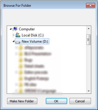
Figure 2
If you haven't previously prepared the directory, you can do it by clicking Make New Folder (Figure 3).
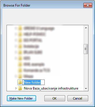
Figure 3
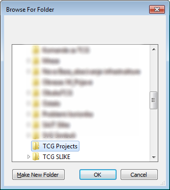
Assign a name to the new directory (in the example, the assigned name is "TCG projects" (Figure 4)).
Figure 4 By clicking OK In “Project Folder” field, now there is a path to the directory determined as "Project Directory" (Figure 4a).
|
Figure 4a |
System Settings
| General Settings | Routing | Copper Cables | Optical Cables | Protective Elements |
General
Settings |
Optical
Single-mode Cable |
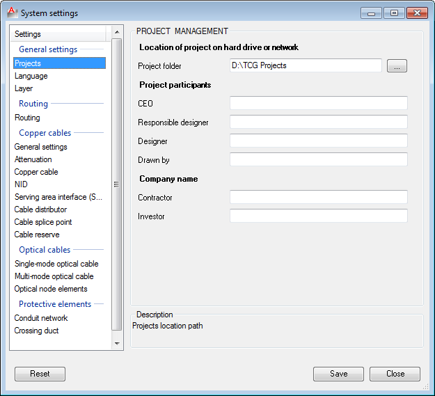
Projects
(Project Management)
Besides the earlier described project directory defining, on this page you also enter data on project development participants and company name. These data will be entered in various forms and at various moments
in the course of the project (offered to the user to be changed
at any time).
|
Figure 5 |
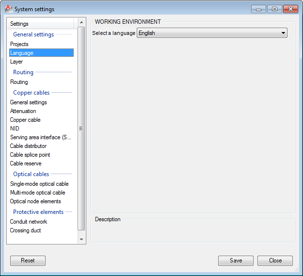
Language
(Working Environment)
On this page the user can choose the TeleCAD-GIS working environment language. From the "Select Language" drop-down list, choose one of the offered languages and record changes by clicking Save. After that, a window pops out informing you that it’s necessary to restart the program for the changes to take effect. You’ll be offered to do it right away. Make sure that, before restarting the program, you save the drawings previously worked on.
|
Figure 6 |
Layer
(Manage Layer Layout)
The default layout of the layers
containing TCG objects is displayed on this page. The user can rearrange the layer layout, after which the new layout becomes the default one. Purpose: The precondition is that each infrastructure type is on its
default layer. If it’s not, you can first run: Note: Procedure:
In the end you need to save changes by clicking on Save. |
Figure 7 |
 -moves to the top of the list
 -moves one place up
 -moves one space down
 -moves to the bottom of the list
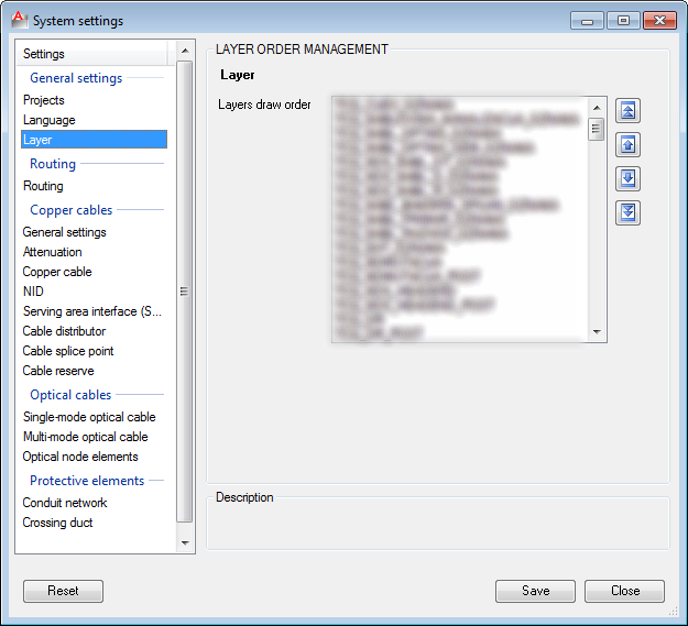
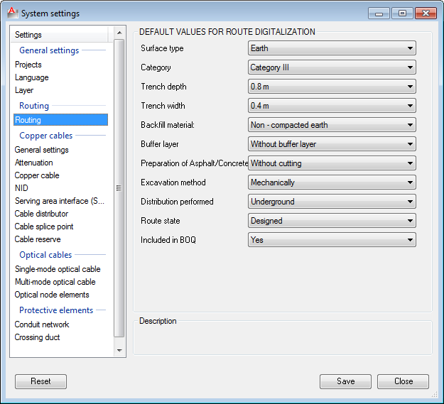
Routing
(Default routing values when digitalising
the route)
When by using Digitised
Route command, Also, if you draw a new route in the drawing, every newly created route segment will be drawn with the properties defined here.
|
Figure 8 |
General Settings
(General Settings for Access Network with
Copper Cables)
General
Settings refer to automatic
numbering method of elements and the layout of the inventory
list. Numeration of elements during automatic processing Elements are numerated in relation to their distance from the telephone exchange. If you selected “Numeration in relation to distribution network elements", then the furthest distribution terminal will be numerated as "1", the next furthest one with "2" and so on. If you selected “Numeration in relation to distribution and drop plant network elements", then the distribution terminal with the furthest NID will be numerated as "1”, distribution terminal with the next furthest NID as “2” etc. Other elements are numerated in
accordance with the specified rule. Inventory list display while being generated for printing (This item is self-explanatory)
|
Figure 9 |

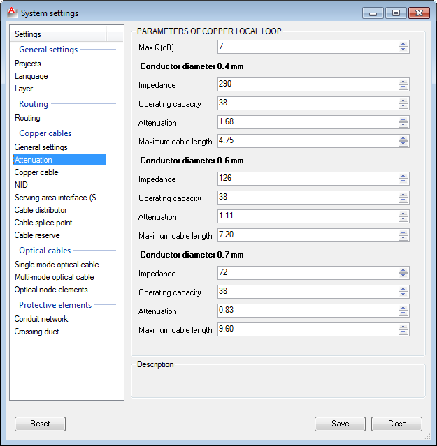
Attenuation
(Parameters of the subscriber copper duct)
These parameters impact the choice of cable conductor diameter when optimising distribution and drop plant network cables. Parameters of the items:
are standard parameters obtained from the manufacturer (the user can modify them). Max Q (dB) is a parameter entered by the user, and it represents the maximum value. The program takes the values given for Q(dB) <= Max Q(dB), during the optimisation cables (We described the procedure when starting with duct diameter 0.4 mm, but in reality you’d start from duct diameter defined on "Copper cable" page (see below))
|
Figure 10 |
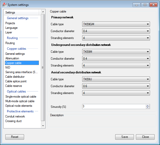
Copper Cable
(Copper cable)
When laying a new cable with one of the commands: the program will lay cables with properties defined on this page.
When calculating the diameter of conductor
In addition, here we define the default value for sinuosity that is also used when laying a new cable.
|
Figure 11 |
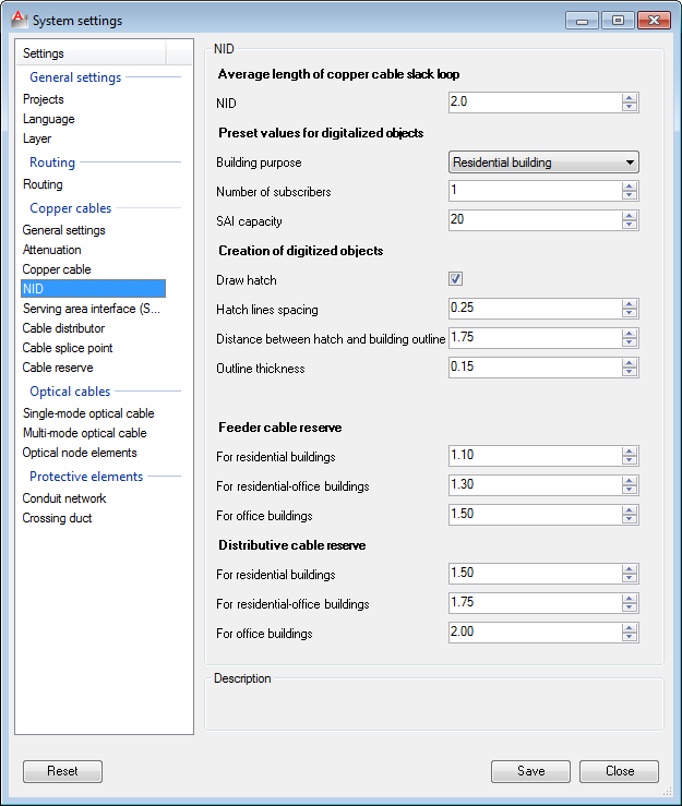
NID (Network interface device)
NID (Network Interface Device)
Average length of copper cable slack loop The user defines the average length of copper cable slack loop , when the cable is laid to the NID (PS or WD). These parameters will be used when drawing a new cable laid to the NID, using one of the commands: Note
Predefined values for digitalised objects The user defines the parameters that will be used when you use the command Digitised Object.
Rendering of digitised objects The user defines whether when drawing the building there’ll be hatching and the appearance of the building symbols.
Slack loop on main directions At this place we define Valid for the commands:
Slack loop on distribution directions Same as the previous item,
(Regarding the use of |
Figure 12 |
Pedestal DT
(Pedestal DT)
On this page the user defines the average length of copper cable slack loop , when the cable is laid to the Pedestal DT. The length can be defined for each type of Pedestal DT separately. These parameters will be used when drawing a new cable laid to the distribution terminal, using one of the commands:
In addition, in the “Pass-through pole” section
Note: |
Figure 13 |
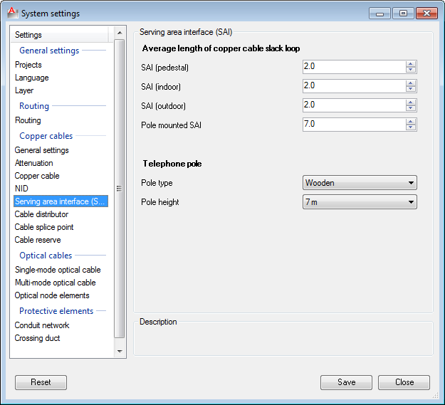
Feeder Distribution Interface
Feeder Distribution Interface
On this page the user defines the average length of the copper cable slack loop, when the cable is laid to the distribution frame. These parameters will be used when drawing a new cable laid to the distribution frame, using one of the commands:
Note: |
Figure 14 |
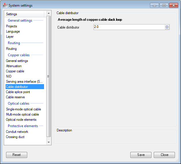
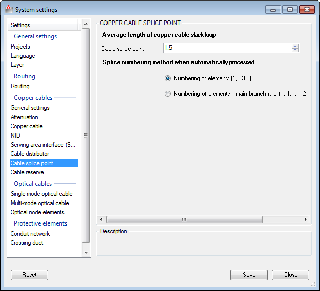
Copper cable splice point
(Copper cable splice point)
On this page the user defines the average length of copper cable slack loop , when the cable is laid to the splice point. These parameters will be used when drawing a new cable laid to (or from) the splice point, using one of the commands:
In addition, on this page we defined the numbering method of the splice point during automatic numbering.
Note: |
Figure 15 |
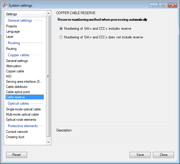
Splice point in copper cable
*(Splice point in copper cable)
On this page we define whether the reserve (in capacity) will be included in the numbering during automatic numbering.
|
Figure 16 |
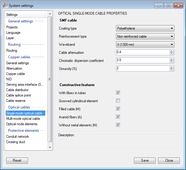
Optical Single-mode Cable
(Properties of Optical Single-mode Cable)
When laying a new TOSM cable, the cable will be laid with properties defined on this page regardless of whether or not the cable is drawn by command: |
Figure 17 |
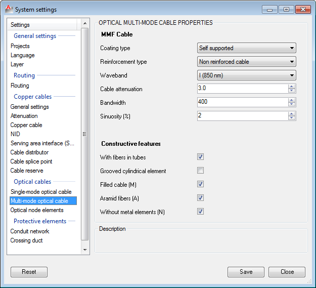
Optical Multi-mode Cable
(Properties of Optical Multi-mode Cable)
When laying a new MMF cable, it will be laid with properties defined on this page, regardless of whether the cable is drawn by command:
|
Figure 18 |
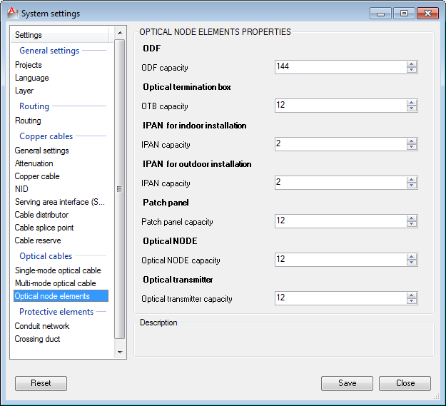
Optical Nodal Elements
(Optical Nodal Elements Properties)
When setting new optical nodal elements, they will be assigned the capacity defined here. For each nodal element there is a minimum capacity that can be assigned:
Modification of nodal elements capacity is described on the Modify Distribution Frame Capacity page.
|
Figure 19 |
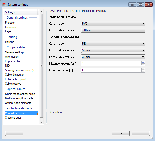
Duct Bank
Duct Bank Basic Properties
Each newly laid duct by command: will have the properties defined in section
will have the properties defined in section |
Figure 20 |
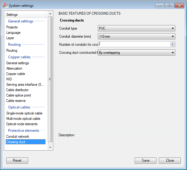
Crossing Ducts
(Basic properties of crossing ducts)
Each newly laid duct by command:
will have the properties defined on this page.
through the selected command.
are taken from here. |
Figure 21 |